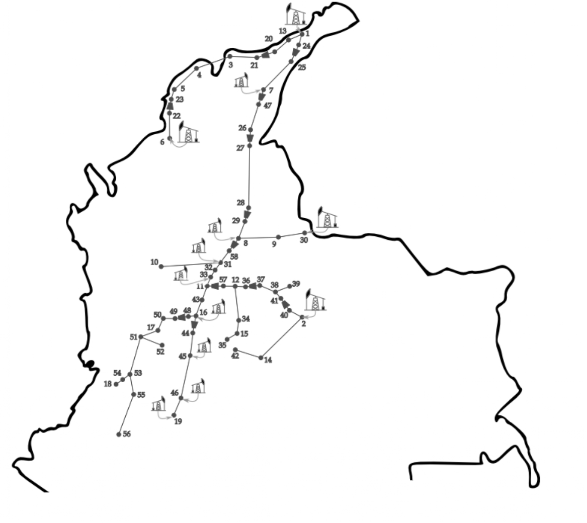
##Implementation in the Colombian gas network with 15 nodes and one source

In this study, an optimization model inspired by the approach presented by García-Marín et al. (2022) is developed. Its purpose is to overcome the limitations of the linear model by incorporating the relationship between flows and pressures. This incorporation transforms the linear model into a nonlinear one, resulting in a more accurate and essential representation of the dynamics in gas distribution networks. This model focuses on the effective management of flows through pipelines and pressures at nodes, systematically addressing the nonlinear complexities and challenges inherent in gas network optimization, as illustrated in the optimization problem with the objective function described below:

Regarding constraints, the optimization problem encompasses various boundary conditions that must be met:

Within this framework, the variables\(f^{\dot{w}} \in \mathbb{R}^{\dot{W} \times 1}\), \(f^{p} \in \mathbb{R}^{P \times 1}\), \(f^{c} \in \mathbb{R}^{C \times 1}\), and \(f^{d} \in \mathbb{R}^{D \times 1}\) denote the gas flows related to injection, transportation, compression, and unsatisfied demand, respectively, where ̇\(\dot{W}\), \(P\), \(C\), and \(D\) signify the number of nodes for each scenario. Conversely, the coefficients \(c^{\dot{w}} \in \mathbb{R}^{1 \times \dot{W}}\), \(c^{p} \in \mathbb{R}^{1 \times P}\), \(c^{c} \in \mathbb{R}^{1 \times C}\), and \(c^{d} \in \mathbb{R}^{1 \times D}\) correspond to the costs associated with each of these flows.

Regarding the constraints, the optimization problem encompasses several boundary conditions that must be met:

\(f^{\dot{w}}_{\text{min}} \leq f^{\dot{w}} \leq f^{\dot{w}}_{\text{max}}\),

\(f^{p}_{\text{min}} \leq f^{p} \leq f^{p}_{\text{max}}\), \(f^{c}_{\text{min}} \leq f^{c} \leq f^{c}_{\text{max}}\), \(0 \leq f^{d} \leq f^{n}\), \(p_{\text{min}} \leq p \leq p_{\text{max}}\)

where the symbols \(f^{\dot{w}}_{\text{min}},f^{\dot{w}}_{\text{max}} \in \mathbb{R}^{\dot{W} \times 1}\), \(f^{p}_{\text{min}},f^{p}_{\text{max}} \in \mathbb{R}^{P \times 1}\), and \(f^{c}_{\text{min}},f^{c}_{\text{max}} \in \mathbb{R}^{C \times 1}\) define the lower and upper bounds for injection, transportation, and compressor flows, respectively. Additionally, \(p, p_{\text{min}}, p_{\text{max}} \in \mathbb{R}^{N \times 1}\) denote the pressures and their respective limits. Finally, \(f^{n} \in \mathbb{R}^{N \times 1}\) represents the system demands at each node, with N being the total number of nodes in the system.

There are three additional fundamental aspects to consider during optimization. The first pertains to node balance, expressed by the equation:

\(mf = f^{n}\)

Here, \(f \in \{f^{\dot{w}},f^{p},f^{c},f^{d}\} \mathbb{R}^{Q \times 1}\) and (m \in `:nbsphinx-math:mathbb{R}`^{N :nbsphinx-math:`times `Q}), with the latter being the incidence matrix encoding the structure of the gas network. The variable (Q) denotes the total number of flows or variables subject to optimization.

The second crucial aspect is the Weymouth constraint, detailed as follows:

$ f^{p}_{i,j} = \text{sgn}`(p_j^2 -p_i^2):nbsphinx-math:sqrt{k_{i,j} |p_j^2 - p_i^2|}` $

Where the subscripts (i, j) indicate the start and end nodes of pipelines, and (k_{i,j}) represents a constant. Lastly, the third aspect, or constraint, is the compression coefficient, formulated as:

$ 1.0 \leq `:nbsphinx-math:frac{p_j}{p_i}` :nbsphinx-math:`leq `b_c $

In this equation, the subscripts (i, j) designate the start and end nodes of compressors, while (b_c) is the compression factor. These elements are crucial for effective optimization and must be addressed meticulously.

from google.colab import files
uploaded = files.upload()

Upload widget is only available when the cell has been executed in the current browser session. Please rerun this cell to enable.

Saving REDCOL (1)_page-0001.jpg to REDCOL (1)_page-0001.jpg

from IPython.display import Image, display

# Ruta de la imagen en tu entorno de Colab
ruta_imagen = 'REDCOL (1)_page-0001.jpg'

# Mostrar la imagen con descripción
display(Image(filename=ruta_imagen, embed=True), metadata={'description': 'RED GAS COLOMBIA'})

Libraries and data for real model

from google.colab import drive
from tensorflow.python.ops.nn_ops import softmax
from keras import backend as k
import numpy as np
from matplotlib.gridspec import GridSpec
from IPython import display
from scipy.optimize import linprog
from sklearn.metrics import mean_squared_error,mean_absolute_error,mean_absolute_percentage_error
import numpy as np
import matplotlib. pyplot as plt
from keras.layers import Activation,Dense,Input,BatchNormalization,Dropout,Conv1D,Flatten,MaxPool1D,Dot,Reshape,Conv2D,Concatenate,ReLU,Lambda,MaxPooling2D,Normalization
import cvxpy as cp
import tensorflow as tf
from keras import Model
from IPython import display
from tensorflow.keras import layers
from tensorflow.keras import regularizers
import warnings
import pandas as pd
from IPython import display
path='/content/drive/MyDrive/Maestría/Optimización/Data/'
from keras.models import Sequential
mse=mean_squared_error
mae=mean_absolute_error
mape=mean_absolute_percentage_error
warnings.filterwarnings("ignore")
drive.mount('/content/drive')
import pandas as pd
import scipy.io as sio
import os
from sklearn.model_selection import train_test_split
from sklearn.preprocessing import MinMaxScaler,StandardScaler
from tensorflow.keras.callbacks import Callback
from typing import Tuple
import matplotlib.pyplot as plt

import os
os.chdir('/content/drive/Shareddrives/red_gas_col/Prueba')
from My_Functions.Object1 import Evaluate,FlyEvaluate
from My_Functions.model_real_data import flow_model, plots, gen_w, plot_time, ng_case_evaluate, ng_evaluate_atip, visualize_atipic, visualize_non_convergence, identify_atypical_values, dynamic_val, loss_val, bounded

Drive already mounted at /content/drive; to attempt to forcibly remount, call drive.mount("/content/drive", force_remount=True).

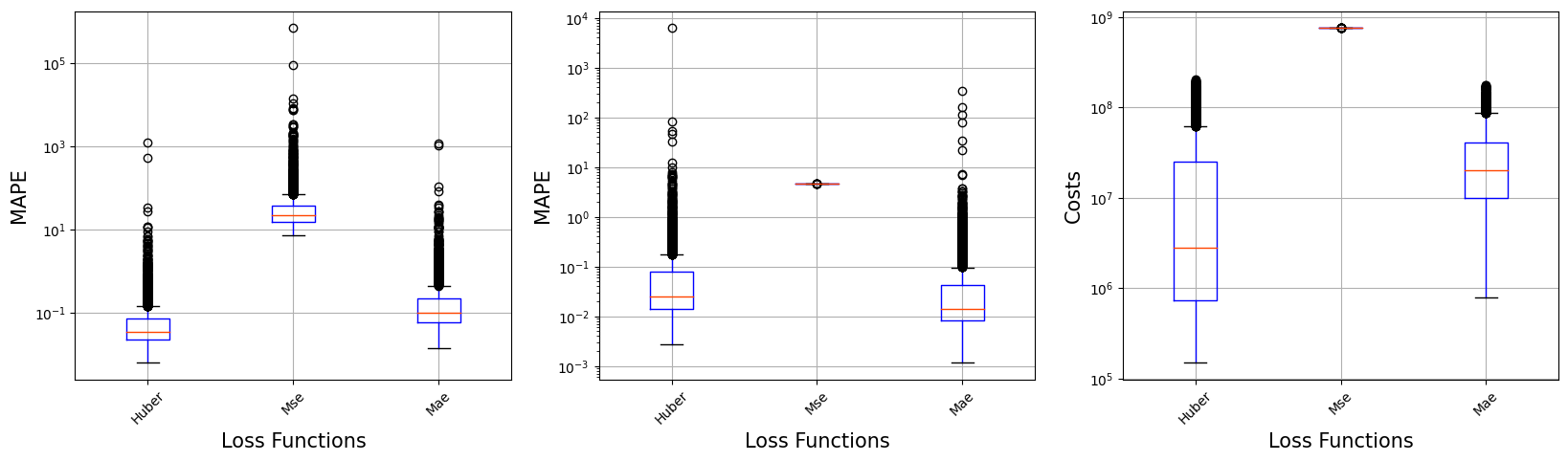
The results indicate that integrating the Huber cost function into the custom cost function for model training improves performance. However, it is essential to evaluate its performance when facing constraints that are considered crucial and complex, such as node balance, the Weymouth equation, and solution-associated costs. For this purpose, the following graph shows the results obtained from evaluating these constraints.

It is evident that Huber tends to produce responses with lower percentage errors in node balance. Although it presents higher errors in the Weymouth equation, overall costs tend to be lower.

loss_val()

#Bounded Restrictions

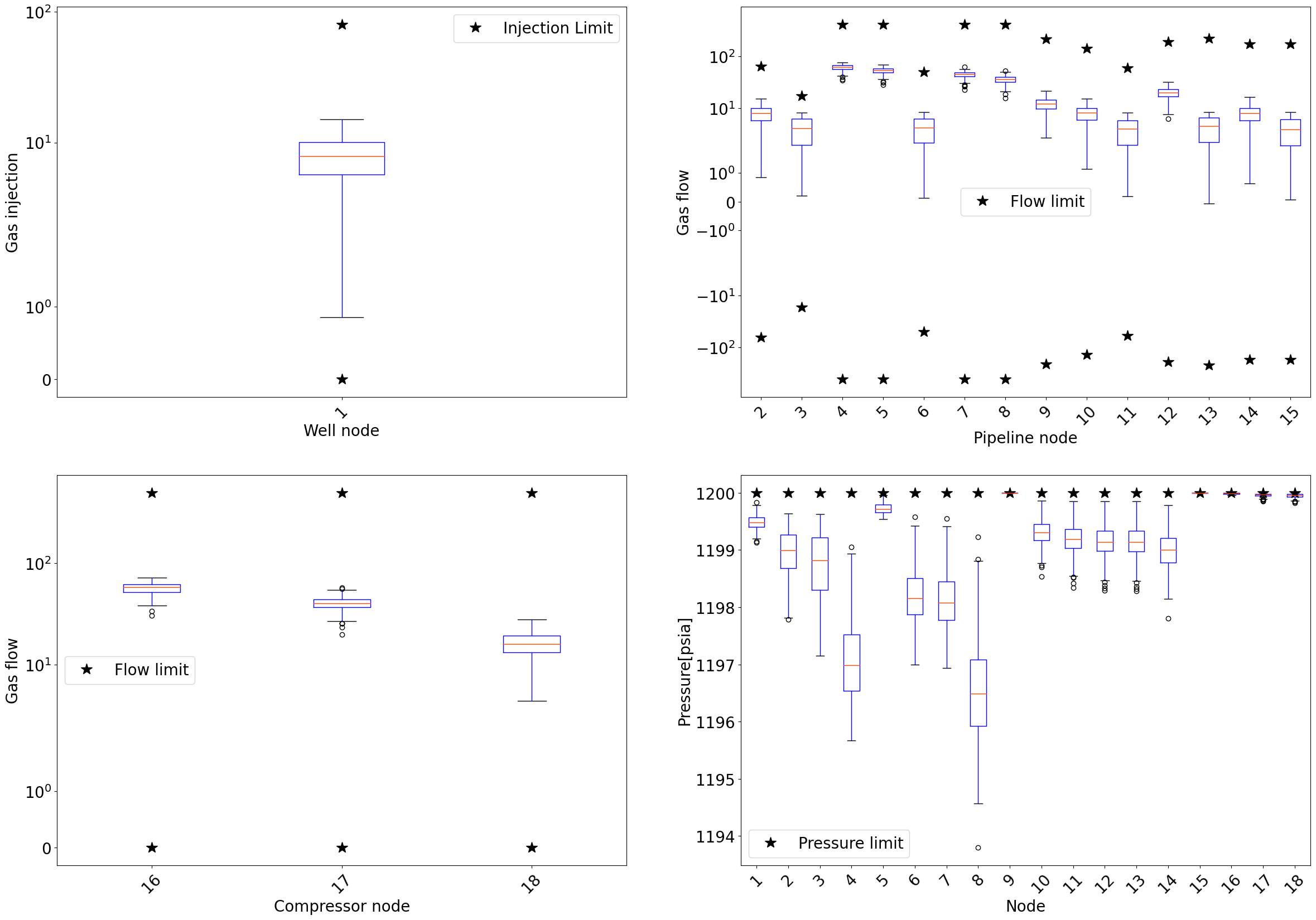
Limit Restriction: This chart shows the behavior of sources, compressors, pipelines and pressures, along with the defined limits for each. The number on the x-axis represents the node, more than an exact number

bounded(s=1)

#Compliance with System Restrictions

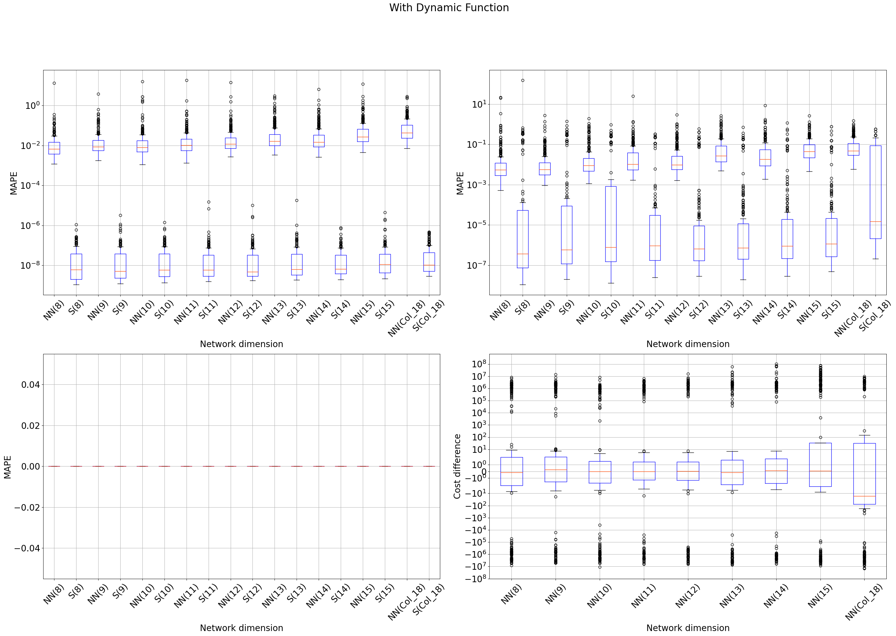
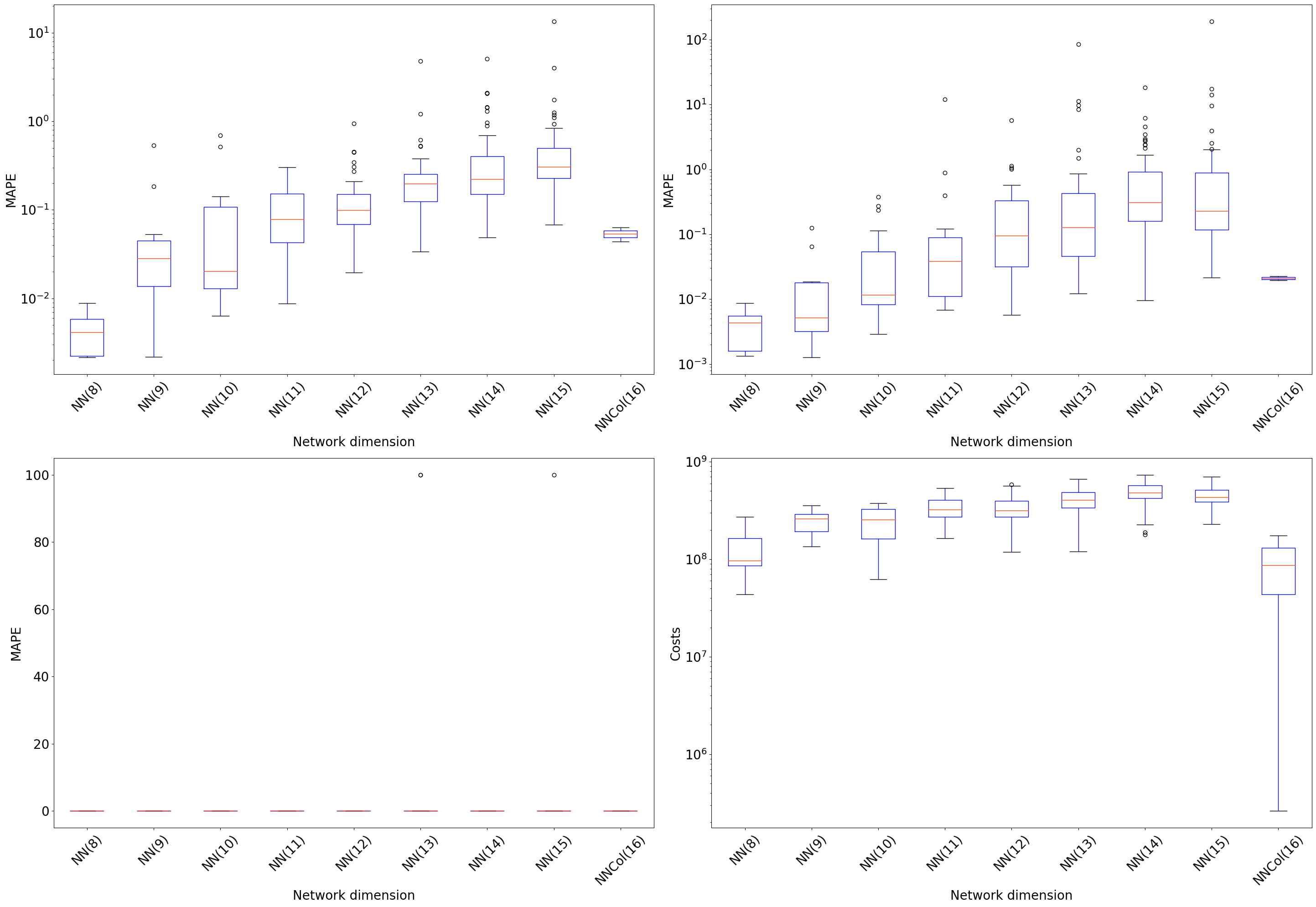
This graph compares the error associated with gas dispatch restrictions, with and without dynamic function, Both graphical representations show the same distribution. The upper left quadrant analyzes the balance of nodes; the upper right, the error in the Weymouth equation; the lower left, the restriction of compression ratio; and the lower right, cost differences between our proposal (NN) and the reference model (S)

Balance,Weymouth,PjPi,Costos=ng_case_evaluate(s=0)

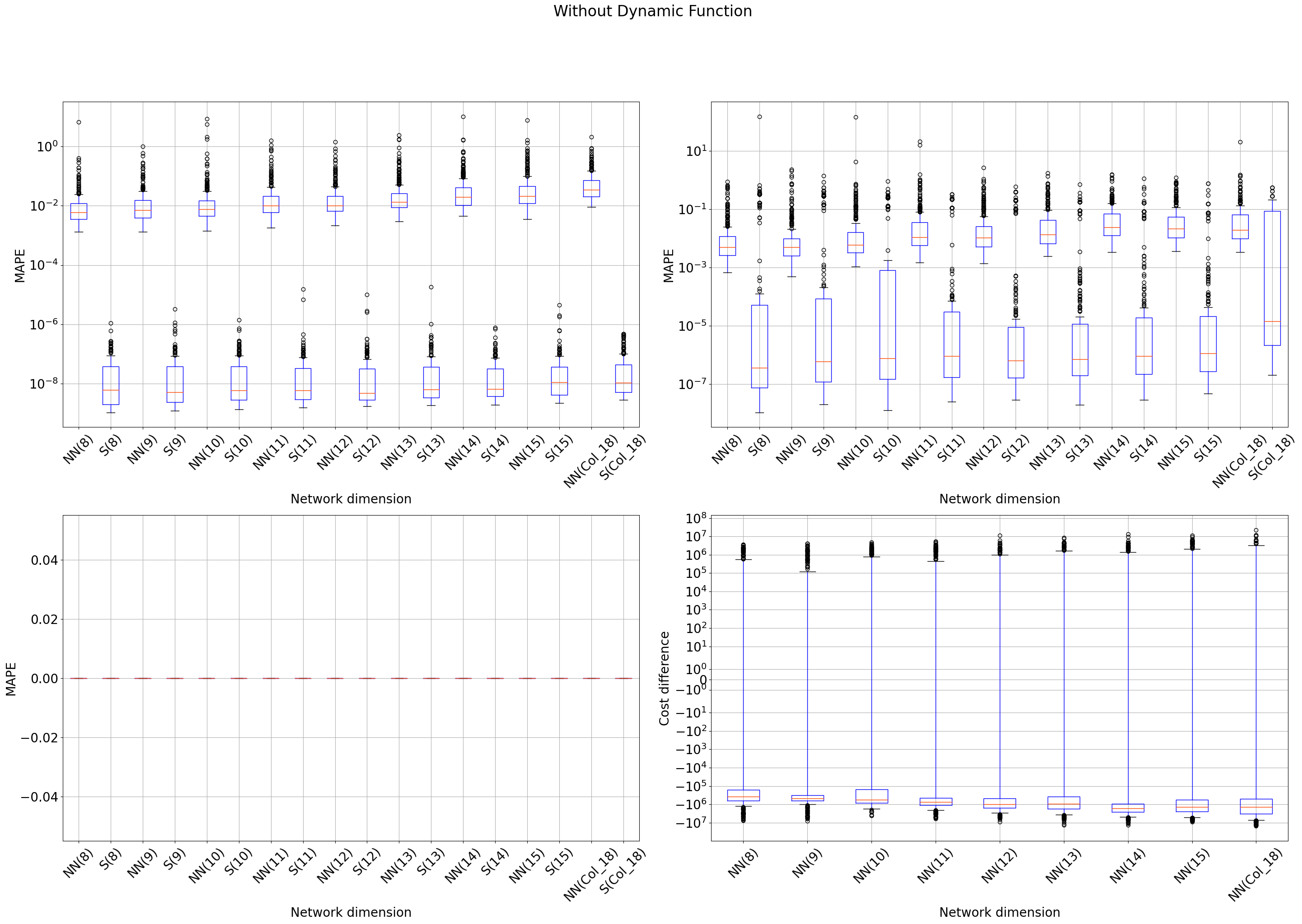
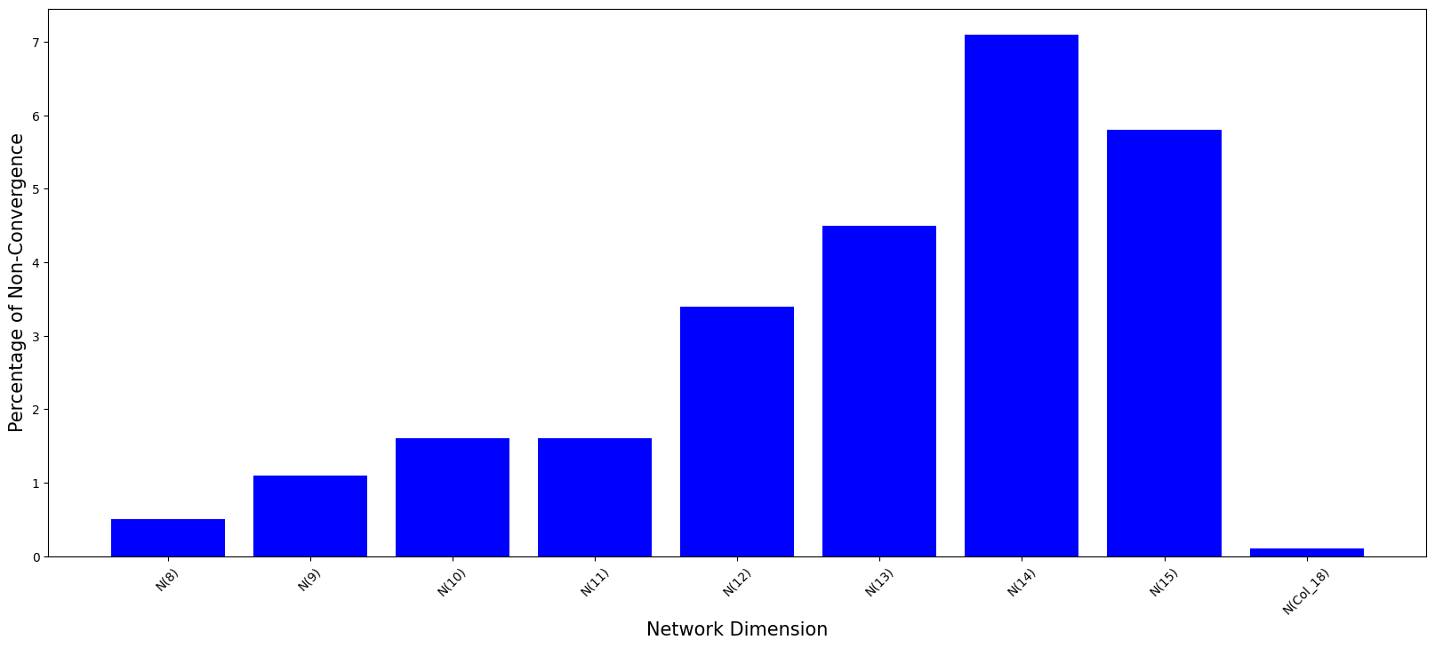
Illustration representing the occurrence of convergence failures in each gas network (N), with numerical values indicating the nodes of each network

visualize_non_convergence()

This graph compares the error associated with gas dispatch restrictions, with and without dynamic function, Both graphical representations show the same distribution. The upper left quadrant analyzes the balance of nodes; the upper right, the error in the Weymouth equation; the lower left, the restriction of compression ratio; and the lower right, cost differences between our proposal (NN) and the reference model (S).

Balance,Weymouth,PjPi,Costos= ng_case_evaluate(s=1)

Outlier Proportion

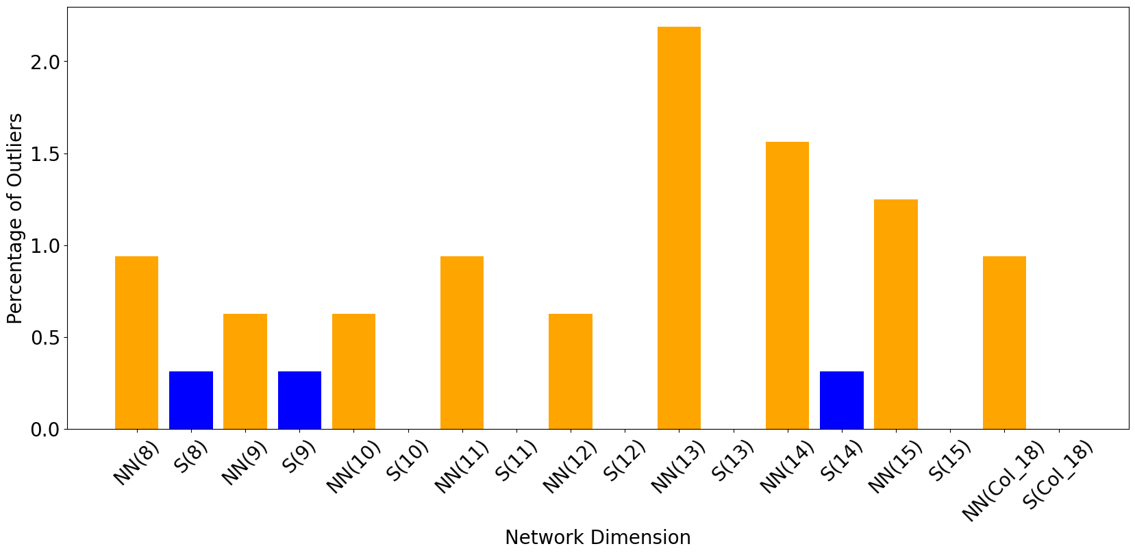
The first graph shows the outliers associated with the node balance equation for both the PINN and the solver, represented by the symbols NN and S, respectively. On the other hand, the second graph illustrates the outliers linked to the Weymouth equation for the PINN and the solver, represented as NN and S respectively.

df=Balance
columnas_red = df.columns#[col for col in df.columns if 'S' in col]
print('Porcentaje de atípicos: Balance de nodos')
visualize_atipic(Balance, columnas_red)
print('Porcentaje de atípicos: Weymouth')
visualize_atipic(Weymouth, columnas_red)

Porcentaje de atípicos: Balance de nodos

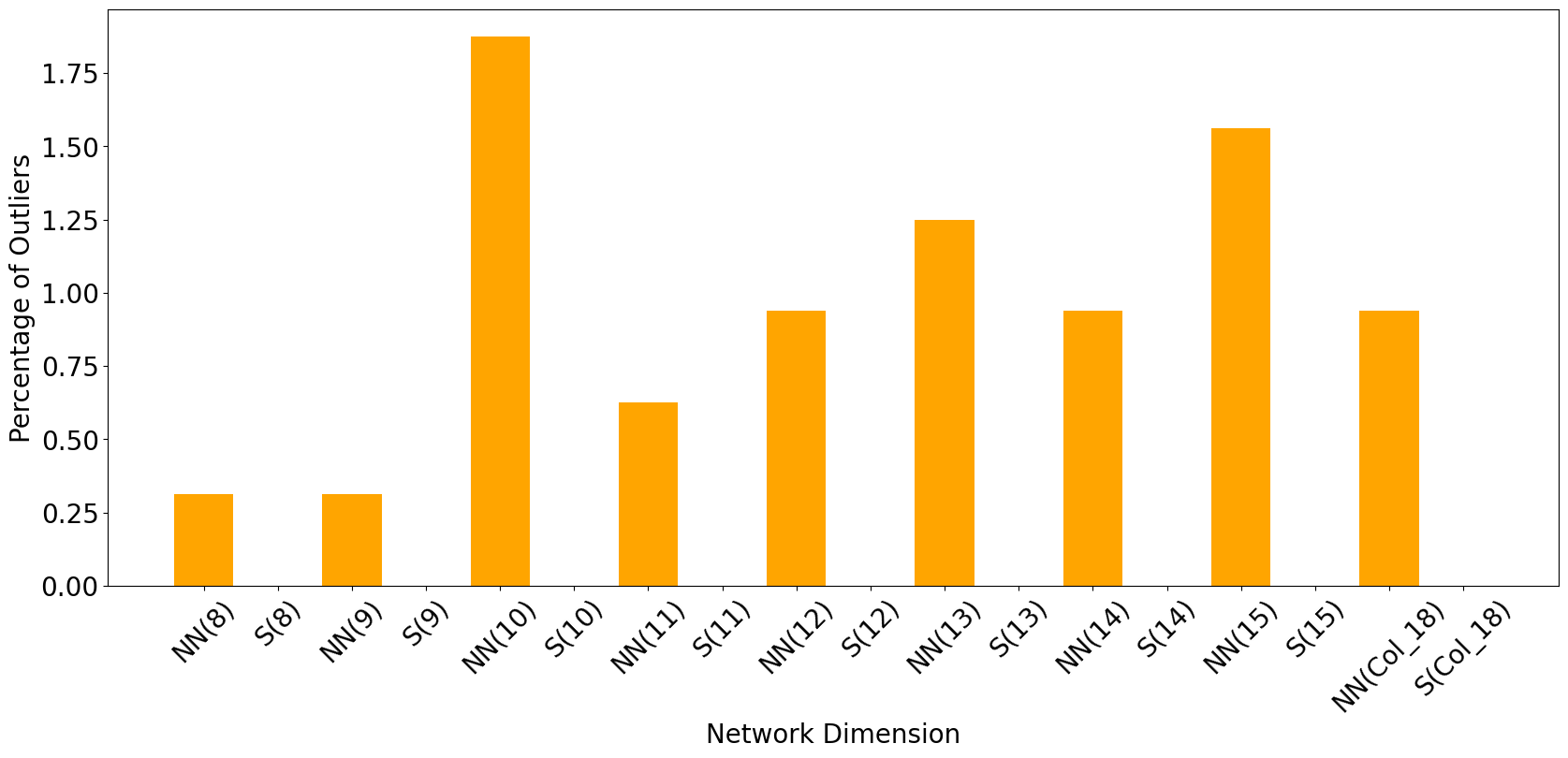
Porcentaje de atípicos: Weymouth

#Computing Time

The comparison diagram depicts the time used by the traditional method vs the time expended by our methodology throughout the training phase to resolve an optimization problem.This diagram employs the letters NN and S to differentiate between our methodology and the conventional approach, respectively.

a=plot_time(s=1)

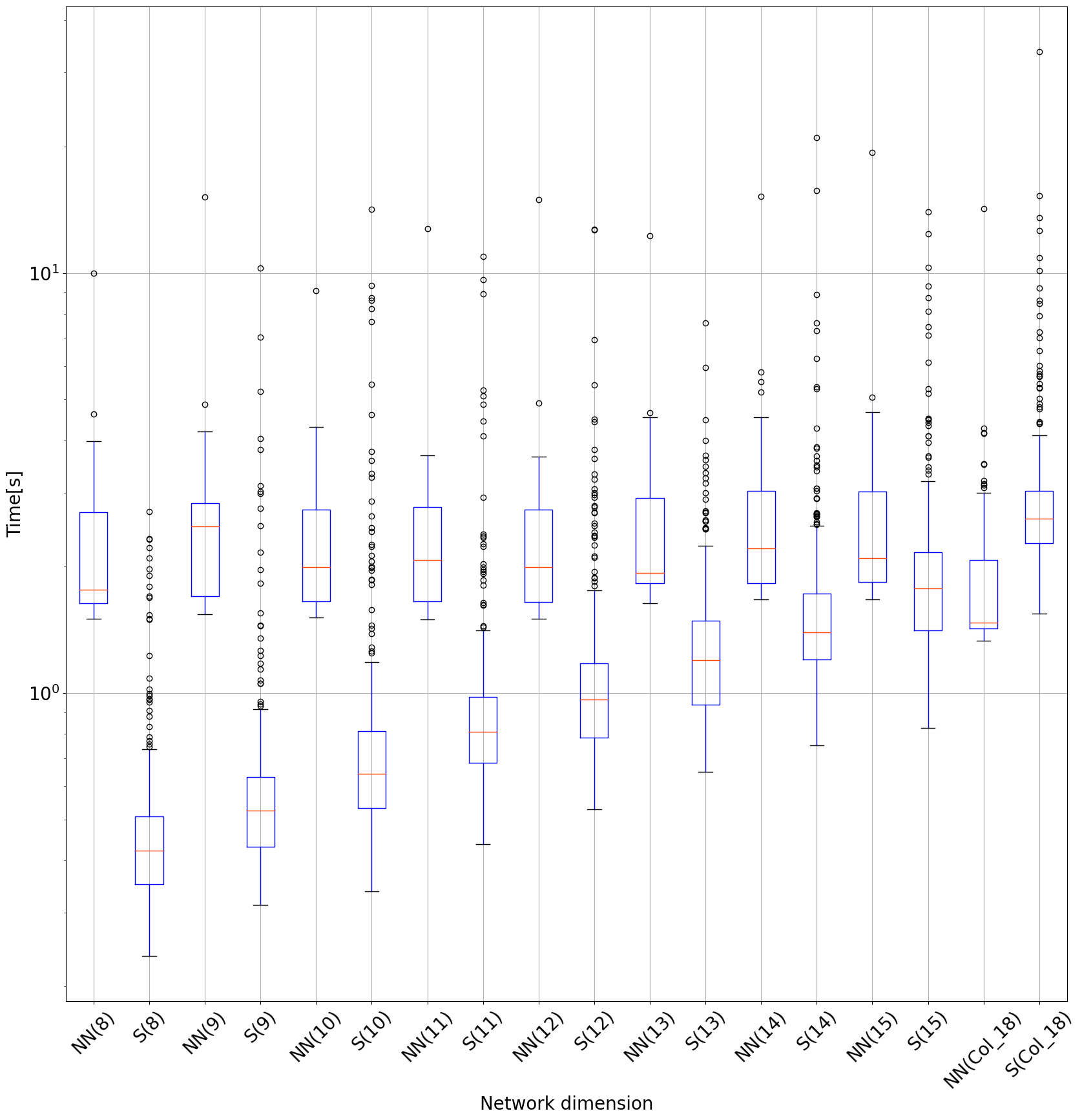
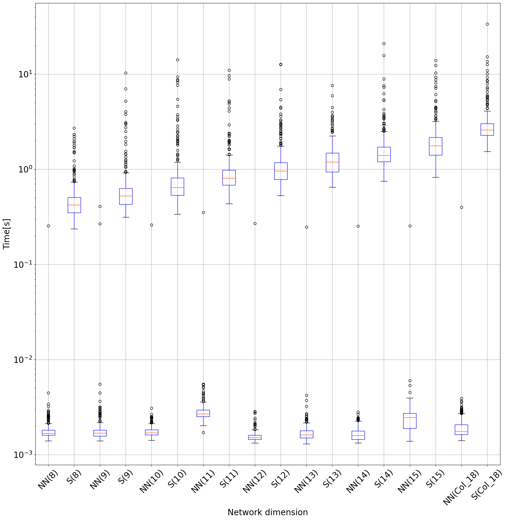
The graph illustrates the comparison of resolution times for test data between the classic technique (marked by the letter S) and our strategy (represented by the letters NN).

a=plot_time('predict',s=1)

Evaluation of the performance of our Neural Network (NN) proposal for gas networks, showing the balance of nodes (on the top left axis), the Weymouth equation (on top right axis) and, on the bottom, the limitation of compression ratio and associated costs

Bal,Wey,_,_=ng_evaluate_atip(s=1)

WARNING:tensorflow:5 out of the last 324 calls to <function Model.make_predict_function.<locals>.predict_function at 0x780a69c1b520> triggered tf.function retracing. Tracing is expensive and the excessive number of tracings could be due to (1) creating @tf.function repeatedly in a loop, (2) passing tensors with different shapes, (3) passing Python objects instead of tensors. For (1), please define your @tf.function outside of the loop. For (2), @tf.function has reduce_retracing=True option that can avoid unnecessary retracing. For (3), please refer to https://www.tensorflow.org/guide/function#controlling_retracing and https://www.tensorflow.org/api_docs/python/tf/function for  more details.
WARNING:tensorflow:6 out of the last 325 calls to <function Model.make_predict_function.<locals>.predict_function at 0x780a6d130a60> triggered tf.function retracing. Tracing is expensive and the excessive number of tracings could be due to (1) creating @tf.function repeatedly in a loop, (2) passing tensors with different shapes, (3) passing Python objects instead of tensors. For (1), please define your @tf.function outside of the loop. For (2), @tf.function has reduce_retracing=True option that can avoid unnecessary retracing. For (3), please refer to https://www.tensorflow.org/guide/function#controlling_retracing and https://www.tensorflow.org/api_docs/python/tf/function for  more details.

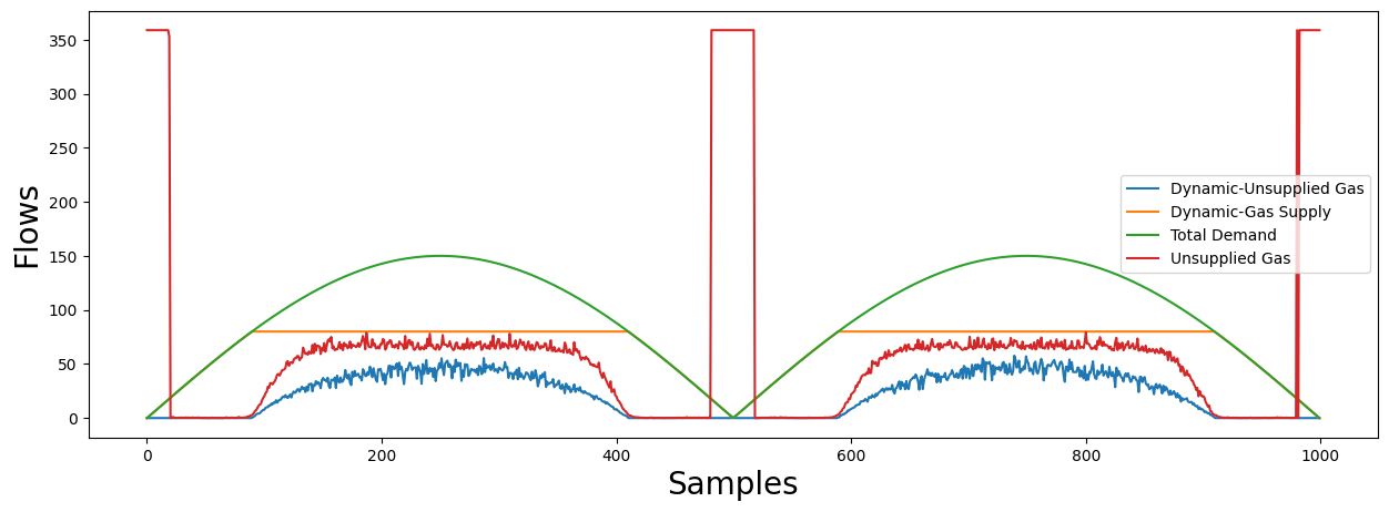
The figure illustrates the behavior of dynamic activation functions in a simulated scenario of oscillating demand. In the figure on the left, the behavior of the injection flow is observed when the source capacity is exceeded, and how unsupplied demand ceases to be zero in this context. On the other hand, to the right, the sum of supply flows with and without the proposed dynamic function is presented

dinamic = dynamic_val()